[1]:
import matplotlib as mpl
import matplotlib.pyplot as plt
import numpy as np
import TransportMaps as TM
from TransportMaps import KL
import TransportMaps.Maps as MAPS
import TransportMaps.Distributions as DIST
mpl.rcParams['font.size'] = 15
Biochemical oxygen demand (BOD)

The following example treat a model for the demand of dissolved oxygen by aerobic biological organism in order to break down organic material in a given water sample. The measurement of this oxygen demand helps to gauge the effectiveness of wastewater treatment plants. See wiki for more informations.
Diagnostics and unbiased sampling
We consider here a Bayesian approach for the inference of the coefficients \(A\) and \(B\) of the biochemical oxygen demand (BOD) model [OR5]:
given a number \(n\) of observations \(D := [\mathfrak{B}(1), \ldots, \mathfrak{B}(n)]\). The model parameters are endowed with the following priors
We consider here the approach introduced in [TM3] which is based on the efficient conditioning of the joint density \((\mathfrak{B}(1), \ldots, \mathfrak{B}(n), A, B) \sim \pi\).
We restrict our attention on the approximation of \((\mathfrak{B}(1), \ldots, \mathfrak{B}(n), A, B) \sim\pi\) and will consider the case \(n=2\) and \(\sigma^2 = 10^{-3}\).
[2]:
import scipy.special

class BODjoint(DIST.Distribution):
    def __init__(self, numY, sigma2 = 1e-3 ):
        sigma = np.sqrt(sigma2)
        timeY=np.arange(numY)+1.
        dimDensity = numY+2
        super(BODjoint,self).__init__(dimDensity)
        self.numY = numY
        self.timeY  = timeY
        self.sigma = sigma
    def pdf(self, x, params=None, *args, **kwargs):
        return np.exp(self.log_pdf(x, params))
    def log_pdf(self, x, params=None, *args, **kwargs):
        # x is a 2-d array of points. The first dimension corresponds to the number of points.
        #The first numY columns of x refer to the data
        numY = self.numY
        Y = x[:,0:numY]
        theta1=x[:,numY] #The last two components refer to the parameters
        theta2=x[:,numY+1]
        a = .4  + .4*( 1 + scipy.special.erf( theta1/np.sqrt(2) )  )
        b = .01 + .15*( 1 + scipy.special.erf( theta2/np.sqrt(2) )  )
        return -1.0/(2*self.sigma**2) * \
            np.sum( (Y - a[:,np.newaxis]*( 1 - np.exp( -np.outer(b, self.timeY) ) ) )**2 , axis=1) + \
            -.5*( theta1**2 + theta2**2 )
    def grad_x_log_pdf(self, x, params=None, *args, **kwargs):
        numY = self.numY
        Y = x[:,0:numY]
        theta1=x[:,numY] #The last two components refer to the parameters
        theta2=x[:,numY+1]
        a = .4  + .4*( 1 + scipy.special.erf( theta1/np.sqrt(2) )  )
        b = .01 + .15*( 1 + scipy.special.erf( theta2/np.sqrt(2) )  )
        da_theta1 = .4*np.sqrt(2/np.pi)*np.exp( -theta1**2/2.)
        db_theta2 = .15*np.sqrt(2/np.pi)*np.exp( -theta2**2/2.)
        grad = np.zeros( x.shape )
        for jj in np.arange(numY):
            grad[:,numY] -= -da_theta1/(self.sigma**2)*( 1 - np.exp( - b*self.timeY[jj])  )*( Y[:,jj] - a*(1- np.exp(-b*self.timeY[jj])) )
            grad[:,numY+1] -= -1.0/(self.sigma**2)*self.timeY[jj]*db_theta2*a*np.exp(-b*self.timeY[jj])*( Y[:,jj] - a*(1- np.exp(-b*self.timeY[jj])) )
            grad[:,jj] = -1.0/self.sigma**2 *( Y[:,jj] - a*(1-np.exp(-b*self.timeY[jj])) )
        grad[:,-2] -=  theta1
        grad[:,-1] -=  theta2
        return grad
    def hess_x_log_pdf(self, x, params=None, *args, **kwargs):
        numY = self.numY
        Y = x[:,0:numY]
        theta1=x[:,numY] #The last two components refer to the parameters
        theta2=x[:,numY+1]
        a = .4  + .4*( 1 + scipy.special.erf( theta1/np.sqrt(2) )  )
        b = .01 + .15*( 1 + scipy.special.erf( theta2/np.sqrt(2) )  )
        da_theta1 = .4*np.sqrt(2/np.pi)*np.exp( -theta1**2/2.)
        db_theta2 = .15*np.sqrt(2/np.pi)*np.exp( -theta2**2/2.)
        d2a_theta1 = -theta1*da_theta1
        d2b_theta2 = -theta2*db_theta2
        Hess_x = np.zeros( (x.shape[0], x.shape[1],  x.shape[1]) )
        for jj in np.arange(numY):
            Hess_x[:,numY,numY]-= -(1-np.exp(-b*self.timeY[jj]))/(self.sigma**2)*( d2a_theta1*( Y[:,jj] - a*(1- np.exp(-b*self.timeY[jj])) ) - da_theta1**2*(1-np.exp(-b*self.timeY[jj]))  )
            Hess_x[:,numY+1,numY]-=  -da_theta1/(self.sigma**2)*( db_theta2*self.timeY[jj]*np.exp(-b*self.timeY[jj])*(Y[:,jj]-a+a*np.exp(-b*self.timeY[jj])) + (1-np.exp(-b*self.timeY[jj]))*(-a*self.timeY[jj]*db_theta2*np.exp(-b*self.timeY[jj])))
            Hess_x[:,numY+1,numY+1]-= -self.timeY[jj]*a/(self.sigma**2)*np.exp(-b*self.timeY[jj])*( ( Y[:,jj] - a*(1- np.exp(-b*self.timeY[jj])) )*( d2b_theta2 - self.timeY[jj]*db_theta2**2 ) - db_theta2**2 *self.timeY[jj]*a*np.exp(-b*self.timeY[jj]))
            Hess_x[:,numY,jj] = da_theta1/(self.sigma**2)*(1-np.exp(-b*self.timeY[jj]))
            Hess_x[:,numY+1,jj] = 1/(self.sigma**2)*self.timeY[jj]*db_theta2*a*np.exp(-b*self.timeY[jj])
            Hess_x[:,jj, numY] = Hess_x[:,numY,jj]
            Hess_x[:,jj, numY+1] = Hess_x[:,numY+1, jj]
        Hess_x[:,numY, numY+1] = Hess_x[:,numY+1, numY]
        Hess_x[:,numY,numY]-=1
        Hess_x[:,numY+1,numY+1]-=1
        for kk in np.arange(x.shape[0]):
            for jj in np.arange(numY):
                Hess_x[ kk , jj, jj]  = -1/(self.sigma**2)
        return Hess_x
[3]:
pi = BODjoint(2, 1e-3)
We can visualize some aligned slices of this \(4\)-dimensional distribution:
[4]:
fig = plt.figure(figsize=(6,6))
varstr=[r"$\mathfrak{B}(1)$", r"$\mathfrak{B}(2)$", r"$A$", r"$B$"]
<Figure size 600x600 with 0 Axes>
[5]:
import TransportMaps.Diagnostics as DIAG
fig = DIAG.plotAlignedConditionals(pi, range_vec=[-4,4],
    numPointsXax=50, fig=fig, show_flag=False, vartitles=varstr)
Integrated squared parametrization
We set up and solve the following variational problem
where \(\mathcal{T}_\triangle\) is in this case the set of integrated squared lower triangular maps. As an initial approximation we use total order expansions with maximum order \(2\) …
[6]:
dim = pi.dim
qtype = 3          # Gauss quadrature
qparams = [6]*dim  # Quadrature order
reg = None         # No regularization
tol = 1e-3         # Optimization tolerance
ders = 2           # Use gradient and Hessian
[7]:
order = 2

T2 = MAPS.assemble_IsotropicIntegratedSquaredTriangularTransportMap(
    dim, order, 'total')

rho = DIST.StandardNormalDistribution( dim )

pull_T2_pi = DIST.PullBackParametricTransportMapDistribution(T2, pi)
push_T2_rho = DIST.PushForwardParametricTransportMapDistribution(T2, rho)

log = KL.minimize_kl_divergence(
    rho, pull_T2_pi, qtype=qtype, qparams=qparams, regularization=reg, tol=tol, ders=ders)
Computing diagnostics
The estimation of the accuracy of an approximation in high dimension is a challenging task, in particular when one seeks approximations to densities which may be unnormalized. These is a typical setting in Bayesian inference and the transport map framework has the remarkable property of providing an asymptotically reliable estimator for such accuracy.
In the following we will present two diagnostics:
the variance diagnostic (formal and quantitative)
the pullback conditionals (informal and qualitative).
Diagnostic routines are contained in the following module:
[8]:
import TransportMaps.Diagnostics as DIAG
Variance diagnostic
As shown in [TM1], as \(\mathcal{D}_{\rm KL}(T_\sharp \nu_\rho \vert \nu_\pi) \rightarrow 0\) (i.e. as \(T\rightarrow T^\star\)), the following holds:
The following code computes this variance diagnostic:
[9]:
pull_T2_pi = DIST.PullBackTransportMapDistribution(T2, pi)
qtype = 0         # Monte-Carlo quadrature
qparams = 1000000 # Number of samples
var_diag = DIAG.variance_approx_kl(
    rho, pull_T2_pi, qtype=qtype, qparams=qparams)
print("Variance diagnostic: %e" % var_diag)
Variance diagnostic: 2.939370e-01
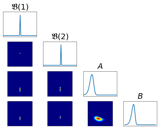
Pullback conditionals
Note that if the transport map \(T\) is accurate, then \(T_\sharp \rho \approx \pi\). Then
where \(\rho\) is the density of \(\mathcal{N}(0,{\bf I})\).
As a consequence, \(T^\sharp \pi\) needs to resemble a Standard Normal distribution, and thus all the n-dimensional conditionals (anchored to \(0\)) will resemble Standard Normals. We use this observation to derive the following qualitative diagnostic, where we plot all the 2-dimensional conditionals of \(T^\sharp \pi\).
[10]:
fig = plt.figure(figsize=(6,6))
varstr = [r"$\mathfrak{B}(1)$", r"$\mathfrak{B}(2)$", r"$A$", r"$B$"]
<Figure size 600x600 with 0 Axes>
[11]:
pull_T2_pi = DIST.PullBackTransportMapDistribution(T2, pi)
fig = DIAG.plotAlignedConditionals( pull_T2_pi, range_vec=[-6,6],
    numPointsXax=50, fig=fig, show_flag=False, vartitles=varstr)

Improving the approximation
As we could see, the obtained approximation performs pretty poorly. Let us try then to improve it using an higher order map, and monitor the improvement using the presented diagnostics.
[12]:
dim = pi.dim
qtype = 3          # Gauss quadrature
qparams = [6]*dim  # Quadrature order
reg = None         # No regularization
tol = 1e-3         # Optimization tolerance
ders = 2           # Use gradient and Hessian
[13]:
order = 3

rho = DIST.StandardNormalDistribution( dim )
T3 = MAPS.assemble_IsotropicIntegratedSquaredTriangularTransportMap(
    dim, order, 'total')
push_rho = DIST.PushForwardParametricTransportMapDistribution(T3, rho)
pull_pi = DIST.PullBackParametricTransportMapDistribution(T3, pi)
# SOLVE
log = KL.minimize_kl_divergence(
    rho, pull_pi, qtype=qtype, qparams=qparams, regularization=reg,
    tol=tol, ders=ders)
Variance diagnostic
[14]:
pull_T3_pi = DIST.PullBackTransportMapDistribution(T3, pi)
qtype = 0         # Monte-Carlo quadrature
qparams = 1000000 # Number of samples
var_diag = DIAG.variance_approx_kl(
    rho, pull_T3_pi, qtype=qtype, qparams=qparams)
print("\nVariance diagnostic: %e" % var_diag)
Variance diagnostic: 1.208082e-01
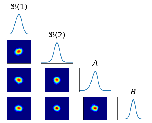
Pullback conditionals
[15]:
fig = plt.figure(figsize=(6,6))
varstr = [r"$\mathfrak{B}(1)$", r"$\mathfrak{B}(2)$", r"$A$", r"$B$"]
<Figure size 600x600 with 0 Axes>
[16]:
pull_T3_pi = DIST.PullBackTransportMapDistribution(T3, pi)
fig = DIAG.plotAlignedConditionals(pull_T3_pi, range_vec=[-6,6],
    numPointsXax=50, fig=fig, show_flag=False, vartitles=varstr)
Unbiased estimators
The approximation of a transport \(\hat{T}_\sharp \nu_\rho \approx \nu_\pi\) is a key ingredient when one wants to perform the integration of a function \(f\) over an intractable distribution \(\nu_\pi\):
The direct sampling of \(\hat{T}_\sharp \nu_\rho\) will introduce some bias in associated estimators due to the residual error. Since \(\hat{T}^\sharp \nu_\pi \approx \nu_\rho\)
we can use \(\nu_\rho\) as an effective biasing (proposal) distribution for \(\hat{T}^\sharp \nu_\pi\)
obtain samples \({\bf X} \sim \hat{T}^\sharp \nu_\pi\)
compute the unbiased samples \(\hat{T}({\bf X})\) from \(\nu_\pi\).
Unbiased sampling routines are contained in the following module:
[17]:
import TransportMaps.Samplers as SAMP
Importance sampling
The importance sampling [OR6] estimator is given by
One can use the sample \(\{{\bf x}_i\}_{i=0}^N \stackrel{\rm iid}{\sim} \rho\) and weights \(w_i = \left. T^\sharp\pi({\bf x}_i) \middle/ \rho({\bf x}_i) \right.\) to obtain the Monte-Carlo approximation
where $:nbsphinx-math:bar`{w}_i = :nbsphinx-math:left`. w_i \middle/ \sum `w_i :nbsphinx-math:right`. $.
If \(\pi \approx c T_\sharp \rho\) then the weights will have little variance
If \(\pi \neq c T_\sharp \rho\) the weights will have a high variance, providing poor estimators.
The form
is preferred to
in this case because it does not involves the evaluation of the density \(T_\sharp \rho({\bf x})\) which requires the sequential inversion (root finding) of the components of \(T\) (this is the case for direct transports, see inverse transports).
We generate \(N=10^4\) importance samples and weights for \(\pi\) using the two approximation of the maps obtained.
The quality of such samples is evaluated looking at the variance of the weights \(\mathbb{V}{\rm ar}[w_i]\), which by definition is strictly related to the variance diagnostic.
[18]:
N = 10000
# Approximation T2
pull_T2_pi = DIST.PullBackTransportMapDistribution(T2, pi)
sampler_T2 = SAMP.ImportanceSampler(pull_T2_pi, rho)
(xt2, wt2) = sampler_T2.rvs(N)
yt2 = T2.evaluate(xt2) # Importance samples from \pi
var_T2 = np.var(wt2) * N
print("Variance weights (T2): %e" % var_T2)
# Approximation T3
pull_T3_pi = DIST.PullBackTransportMapDistribution(T3, pi)
sampler_T3 = SAMP.ImportanceSampler(pull_T3_pi, rho)
(xt3, wt3) = sampler_T3.rvs(N)
yt3 = T3.evaluate(xt3) # Importance samples from \pi
var_T3 = np.var(wt3) * N
print("Variance weights (T3): %e" % var_T3)
Variance weights (T2): 5.405195e-04
Variance weights (T3): 5.078698e-04
Metropolis Hastings with independent proposals
A similar approach to obtain unbiased estimators is to generate a Markov chain with the target distribution \(\nu_\pi\) as invariant distribution.
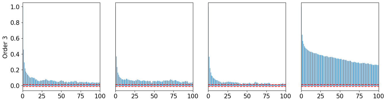
If in importance sampling we obtained an unbiased estimator at the expense of some variance in the weights, here we do it at the expense of independency (not an iid sample). Thus the quality of the sample can be assessed looking at the decay of autocorrelation of the sample.
We use a very basic MCMC sampler (Metropolis Hastings with independent proposals [OR6]):
generate a Markov chain (MC) with
invariant distribution \(\hat{T}^\sharp \nu_\pi\)
using proposal distribution \(\nu_\rho\)
push forward the MC through T obtaining a MC with
invariant distribution \(\nu_\pi\).
The following code generates a Markov Chain of \(N=10000\) samples…
[19]:
burnin = 5000
N = 20000
# Approximation T2
pull_T2_pi = DIST.PullBackTransportMapDistribution(T2, pi)
sampler_T2 = SAMP.MetropolisHastingsIndependentProposalsSampler(
    pull_T2_pi, rho)
(xt2, _) = sampler_T2.rvs(N)
xt2 = xt2[burnin:,:]
yt2 = T2.evaluate(xt2) # Markov chain from \pi
# Approximation T3
pull_T3_pi = DIST.PullBackTransportMapDistribution(T3, pi)
sampler_T3 = SAMP.MetropolisHastingsIndependentProposalsSampler(
    pull_T3_pi, rho)
(xt3, _) = sampler_T3.rvs(N)
xt2 = xt2[burnin:,:]
yt3 = T3.evaluate(xt3) # Markov chain from \pi
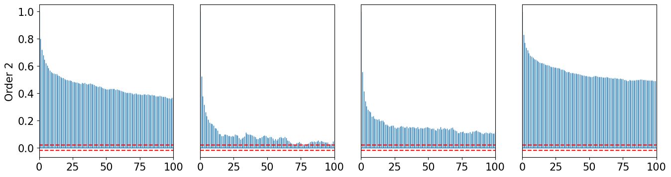
… let’s check the quality of the chain by means of the autocorrelation …
[20]:
def plot_acorr(x, LAGS, title):
    plt.figure(figsize=(16,4))
    nsamps = x.shape[0]
    for d in range(dim):
        ax = plt.subplot(1,dim,d+1)
        s = x[:,d] - np.mean(x[:,d])
        _ = ax.acorr(s, usevlines=True, normed=True, maxlags=LAGS, lw=1)
        var = 1. / np.arange(nsamps, nsamps-LAGS-1, -1)
        cnfint = 1.96 * np.sqrt(var)
        _ = ax.plot(np.arange(LAGS+1), cnfint, '--r')
        _ = ax.plot(np.arange(LAGS+1), -cnfint, '--r')
        ax.set_xlim(0,LAGS)
        if d == 0:
            ax.set_ylabel(title)
        if d > 0:
            ax.get_yaxis().set_visible(False)
[21]:
plot_acorr(xt2, 100, "Order 2")
plot_acorr(xt3, 100, "Order 3")
[22]:
def plot_xcorr(x, LAGS):
    plt.figure(figsize=(6,6))
    nsamps = x.shape[0]
    for d1 in range(dim):
        for d2 in range(d1+1):
            ax = plt.subplot(dim,dim,(d1*dim)+d2+1)
            _ = ax.xcorr(x[:,d1], x[:,d2], usevlines=True, normed=True, maxlags=LAGS, lw=0.3)
            var = 1. / np.arange(nsamps, nsamps-LAGS-1, -1)
            cnfint = 1.96 * np.sqrt(var)
            _ = plt.plot(np.arange(LAGS+1), cnfint, '--r', lw=0.5)
            _ = plt.plot(np.arange(LAGS+1), -cnfint, '--r', lw=0.5)
            ax.set_xlim(0,LAGS)
            ax.set_ylim(-1, 1)
            if d2 > 0:
                ax.get_yaxis().set_visible(False)
            if d1 < dim-1:
                ax.get_xaxis().set_visible(False)
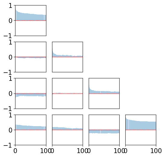
… Let’s check the crosscorrelation between components for order 2 …
[23]:
plot_xcorr(xt2, 100)
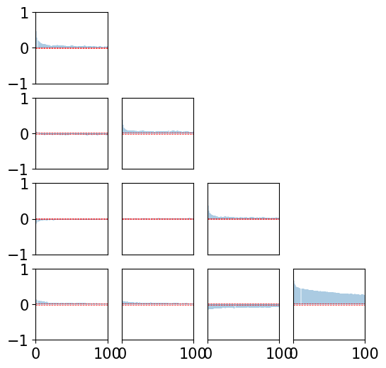
… Let’s check the crosscorrelation between components for order 3 …
[24]:
plot_xcorr(xt3, 100)
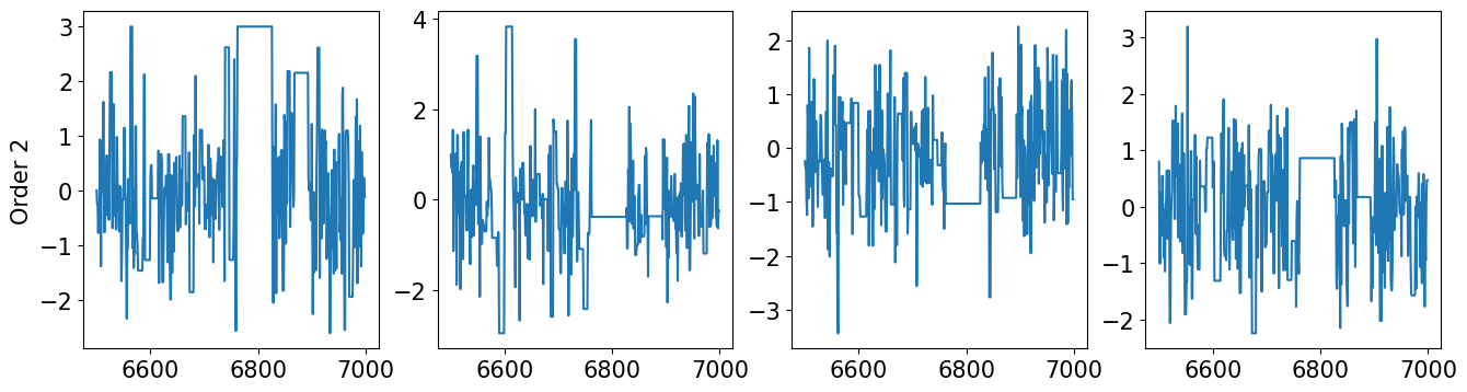
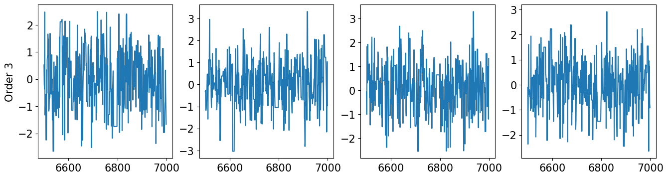
… finally let’s check the mixing of the two chains …
[27]:
def plot_mixing(x, start, stop, title):
    plt.figure(figsize=(16,4))
    nsamps = x.shape[0]
    for d in range(dim):
        ax = plt.subplot(1,dim,d+1)
        _ = ax.plot(range(start,stop),x[start:stop,d])
        if d == 0:
            ax.set_ylabel(title)
[28]:
plot_mixing(xt2, 6500, 7000, "Order 2")
plot_mixing(xt3, 6500, 7000, "Order 3")
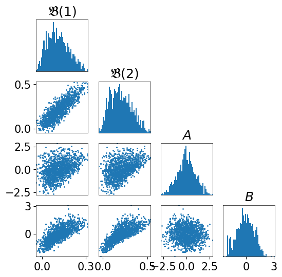
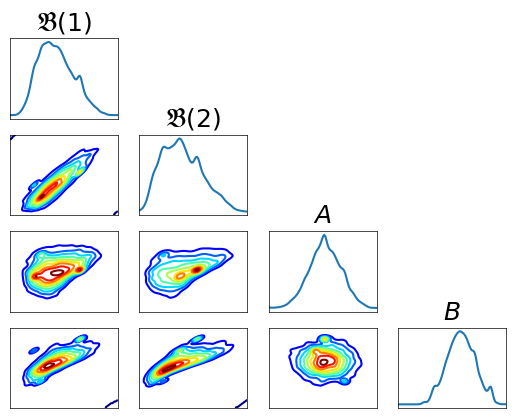
Plotting marginals
[29]:
fig = plt.figure(figsize=(6,6));
<Figure size 600x600 with 0 Axes>
[30]:
fig = DIAG.plotAlignedMarginals(
    yt3, vartitles=varstr, fig=fig, show_flag=False,
    figname='./Figures/BOD/BODmarginals.pdf')
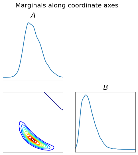
[31]:
fig = plt.figure(figsize=(6,6));
varstr_cond = [r"$A$", r"$B$"]
ncnd_smp = 10000
smp = np.zeros((ncnd_smp,4))
smp[:,:2] = yt3[5000,:2]
rho2 = DIST.StandardNormalDistribution(2)
smp[:,2:] = rho2.rvs(ncnd_smp)
push_smp = T3.evaluate(smp)
fig = DIAG.plotAlignedMarginals(
    push_smp[:,2:],
    vartitles=varstr_cond, fig=fig, show_flag=False,
    figname='./Figures/BOD/BODcond-marginals.pdf')
[32]:
fig = plt.figure(figsize=(6,6));
fig = DIAG.plotAlignedScatters(
    yt3[5000:7000,:], s=1, bins=50, vartitles=varstr,
    fig=fig, show_flag=False)