[1]:
import TransportMaps as TM
import matplotlib
import matplotlib.pyplot as plt
import numpy as np
import TransportMaps.Algorithms.SparsityIdentification as SI
import TransportMaps.Distributions.FrozenDistributions as FD
%matplotlib inline
Sparsity identification algorithm (SING)
In this example we will show how to use the SING algorithm to identify the Markov random field (MRF) corresponding to a given dataset [TM5]. The MRF is encoded with an undirected graph \(\mathcal{G} = (V,E)\). Given data from an unknown distribution \(\pi\), SING learns the conditional independence by estimating the sparsity of a generalized precison matrix \(\Omega = \mathbb{E}_{\pi}[|\partial_{i} \partial_{j} \log \pi|]\). The nonzero entries in \(\Omega\) correspond to edges in \(E\).
To learn the graph, the SING algorithm performs the following steps: - Learns a map from samples - Computes and thresholds \(\Omega\) (setting \(\Omega_{ij} = 0\) is equivalent to \(e_{ij} \notin E\)) - Reorders the variables according to natural ordering - Recomputes map given a sparse candidate graph - Iterates…
Here we have an example of 1000 data points generated from a \(p = 5\) dimensional multivariate normal with a chain graph structure.
[2]:
n_samps = 1000
p = 5
chain_dist = FD.ChainGraphGaussianDistribution(p)
data = chain_dist.rvs(n_samps)
In addition to the dataset, the input parameters to SING are (1) order: the polynomial order used in the parameterization of the map; (2) ordering: the ordering heuristic used to reorder the variables; and (3) delta: a tuning parameter used in the thresholding step.
If the data is from a multivariate normal distribution, using linear maps is sufficient. This corresponds to setting the order to 1. If the data is non-Gaussian, we can use a higher order to better characterize the distribution.
To order the variables, available heuristics are SI.MinFill(), SI.MinDegree(), and SI.ReverseCholesky(). We have found the reverse Cholesky to work well in practice.
Increasing delta promotes sparsity in \(\Omega\). However, this also has the risk of removing edges in the true graph. Typical values for delta lie in the range \([1,5]\). For more information on the effect of varying delta, see [TM5].
[3]:
order = 1
ordering = SI.ReverseCholesky()
delta = 2
generalized_precision = SI.SING(data, order, ordering, delta)
Problem inputs:

 dimension =  5
 number of samples =  1000
 polynomial order =  1
 ordering type =  <class 'TransportMaps.Algorithms.SparsityIdentification.NodeOrdering.ReverseCholesky'>
 delta =  2


SING Iteration:  1
Active variables:  [[0], [0, 1], [0, 1, 2], [1, 3], [0, 4]]
  Note variables may be permuted.
Number of edges:  5  out of  10  possible

SING Iteration:  2
Active variables:  [[0], [0, 1], [0, 2], [2, 3], [3, 4]]
  Note variables may be permuted.
Number of edges:  4  out of  10  possible

SING Iteration:  3
Active variables:  [[0], [0, 1], [0, 2], [2, 3], [3, 4]]
  Note variables may be permuted.
Number of edges:  4  out of  10  possible

SING has terminated.
Total permutation used:  [3 4 2 1 0]
Recovered graph:
 [[ 1.  1.  0.  0.  0.]
 [ 1.  1.  1.  0.  0.]
 [ 0.  1.  1.  1.  0.]
 [ 0.  0.  1.  1.  1.]
 [ 0.  0.  0.  1.  1.]]
At each iteration, SING prints the list of active variables. These variables indicate the functional dependence of each map component.
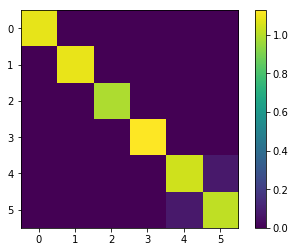
SING returns the generalized precision, as shown below. The non-zeros in this matrix correspond to the edges of the graph. The recovered tri-diagonal structure shows that SING correctly learned the chain graph of the data.
[6]:
generalized_precision
[6]:
array([[ 1.39024902,  0.79365777,  0.        ,  0.        ,  0.        ],
       [ 0.79365777,  1.93068186,  0.92532806,  0.        ,  0.        ],
       [ 0.        ,  0.92532806,  2.14197399,  0.88885174,  0.        ],
       [ 0.        ,  0.        ,  0.88885174,  1.97823071,  0.81248244],
       [ 0.        ,  0.        ,  0.        ,  0.81248244,  1.56063022]])
[7]:
plt.figure()
plt.imshow(generalized_precision)
plt.colorbar()
[7]:
<matplotlib.colorbar.Colorbar at 0x7f8480569320>
Non-Gaussian data
Let’s now try a non-Gaussian dataset of \(2000\) samples from a \(p=6\) dimensional butterfly distribution. This distribution is made up of pairs of random variables. For each pair \((X,Y)\), we take \(X \sim \mathcal{N}(0,1)\), \(Y = WX\) where \(W \sim \mathcal{N}(0,1)\).
[43]:
p = 6
n_samps = 2000
butterfly = FD.ButterflyDistribution(p)
data = butterfly.rvs(n_samps)

plt.scatter(data[:,0],data[:,1])
[43]:
<matplotlib.collections.PathCollection at 0x7f8480166518>
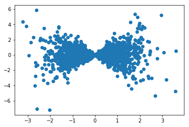
Above is a scatter plot of the first two variables, with a clearly non-Gaussian 2D marginal distribution. Thus, we use order 3 polynomials to capture the non-Gaussian features.
[52]:
order = 3
ordering = SI.ReverseCholesky()
delta = 3
generalized_precision = SI.SING(data, order, ordering, delta)
Problem inputs:

 dimension =  6
 number of samples =  2000
 polynomial order =  3
 ordering type =  <class 'TransportMaps.Algorithms.SparsityIdentification.NodeOrdering.ReverseCholesky'>
 delta =  3


SING Iteration:  1
Active variables:  [[0], [0, 1], [2], [2, 3], [4], [4, 5]]
  Note variables may be permuted.
Number of edges:  3  out of  15  possible

SING Iteration:  2
Active variables:  [[0], [0, 1], [2], [2, 3], [4], [4, 5]]
  Note variables may be permuted.
Number of edges:  3  out of  15  possible

SING has terminated.
Total permutation used:  [0 1 2 3 4 5]
Recovered graph:
 [[ 1.  1.  0.  0.  0.  0.]
 [ 1.  1.  0.  0.  0.  0.]
 [ 0.  0.  1.  1.  0.  0.]
 [ 0.  0.  1.  1.  0.  0.]
 [ 0.  0.  0.  0.  1.  1.]
 [ 0.  0.  0.  0.  1.  1.]]
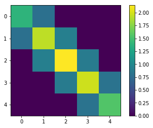
[53]:
plt.figure()
plt.imshow(generalized_precision)
plt.colorbar()
[53]:
<matplotlib.colorbar.Colorbar at 0x7f847ffd8eb8>
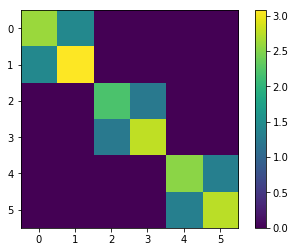
SING correctly recovers the 2x2 block structure of the generalized precision, showing edges between variable pairs. If we try an order 1 map, we incorrectly recover an approximately diagonal \(\Omega\) matrix.
[57]:
order = 1
delta = 3
generalized_precision = SI.SING(data, order, ordering, delta)
Problem inputs:

 dimension =  6
 number of samples =  2000
 polynomial order =  1
 ordering type =  <class 'TransportMaps.Algorithms.SparsityIdentification.NodeOrdering.ReverseCholesky'>
 delta =  3


SING Iteration:  1
Active variables:  [[0], [1], [2], [3], [4], [4, 5]]
  Note variables may be permuted.
Number of edges:  1  out of  15  possible

SING Iteration:  2
Active variables:  [[0], [1], [2], [3], [4], [4, 5]]
  Note variables may be permuted.
Number of edges:  1  out of  15  possible

SING has terminated.
Total permutation used:  [0 1 2 3 4 5]
Recovered graph:
 [[ 1.  0.  0.  0.  0.  0.]
 [ 0.  1.  0.  0.  0.  0.]
 [ 0.  0.  1.  0.  0.  0.]
 [ 0.  0.  0.  1.  0.  0.]
 [ 0.  0.  0.  0.  1.  1.]
 [ 0.  0.  0.  0.  1.  1.]]
[58]:
plt.figure()
plt.imshow(generalized_precision)
plt.colorbar()
[58]:
<matplotlib.colorbar.Colorbar at 0x7f847ff1b518>