import logging
import matplotlib.pyplot as plt
import numpy as np
import scipy.stats as stats
import SpectralToolbox.Spectral1D as S1D
import TransportMaps as TM
import TransportMaps.Maps.Functionals as FUNC
import TransportMaps.Maps as MAPS
from TransportMaps import KL
TM.setLogLevel(logging.INFO)

Inverse transport

Let \(\{x_i\}_{i=1}^\infty\) be a Monte-Carlo sample of a random variable \(X\) with unknown distribution \(\nu_\pi\). Our goal is to characterize this distribution, given a finite sample \(\{x_i\}_{i=1}^n\) from \(X\). We then look for the map \(\hat{S}\) such that

\[\hat{S} = \arg\min_{S\in\mathcal{T}_\triangle} \mathcal{D}_{\rm KL} \left( S_\sharp \nu_\pi \middle\Vert \nu_\rho \right) \;,\]

where \(\nu_\rho\) is the distribution \(\mathcal{N}(0,1)\).

For the sake of this sythetic example we enforce \(X\sim \text{Gumbel}(\mu, \beta)\), with \(\mu=3\) and \(\beta=4\). Let us then construct the Distribution \(\nu_\pi\), for which we are only able to define its (Monte-Carlo) quadrature method (note that in the inference case we instead defined its density).

import TransportMaps.Distributions as DIST

class GumbelDistribution(DIST.Distribution):
    def __init__(self, mu, beta):
        super(GumbelDistribution,self).__init__(1)
        self.mu = mu
        self.beta = beta
        self.dist = stats.gumbel_r(loc=mu, scale=beta)
    def quadrature(self, qtype, qparams, *args, **kwargs):
        if qtype == 0: # Monte-Carlo
            x = self.dist.rvs(qparams)[:,np.newaxis]
            w = np.ones(qparams)/float(qparams)
        else: raise ValueError("Quadrature not defined")
        return (x, w)

mu = 3.
beta = 4.
pi = GumbelDistribution(mu,beta)

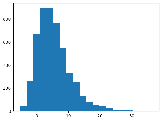
We can then generate and visualize a finite sample…

x, w = pi.quadrature(0, 5000)
plt.figure()
plt.hist(x, bins=20);

For the sake of the example, let us define the complete Gumbel distributions (including its pdf)

class GumbelDistribution(DIST.Distribution):
    def __init__(self, mu, beta):
        super(GumbelDistribution,self).__init__(1)
        self.mu = mu
        self.beta = beta
        self.dist = stats.gumbel_r(loc=mu, scale=beta)
    def pdf(self, x, params=None):
        return self.dist.pdf(x).flatten()
    def quadrature(self, qtype, qparams, *args, **kwargs):
        if qtype == 0: # Monte-Carlo
            x = self.dist.rvs(qparams)[:,np.newaxis]
            w = np.ones(qparams)/float(qparams)
        else: raise ValueError("Quadrature not defined")
        return (x, w)
pi = GumbelDistribution(mu,beta)

Let us also define the exact transport \(S^\star\) such that \(S^\star_\sharp \nu_\pi = \nu_\rho\) …

class GumbelTransportMap(object):
    def __init__(self, mu, beta):
        self.ref = stats.gumbel_r(loc=mu, scale=beta)
        self.tar = stats.norm(0.,1.)
    def evaluate(self, x, params=None):
        if isinstance(x,float):
            x = np.array([[x]])
        if x.ndim == 1:
            x = x[:,NAX]
        out = self.tar.ppf( self.ref.cdf(x) )
        return out
    def __call__(self, x):
        return self.evaluate(x)
Sstar = GumbelTransportMap(mu,beta)

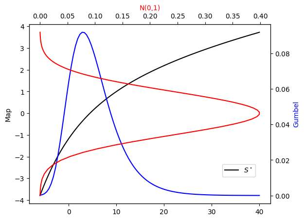
Let us visualize \(S^\star\) and its application on \(\nu_\pi\) …

x_tm = np.linspace(-6,40,100).reshape((100,1))
def plot_mapping(pi_star, Sstar, pi=None, S=None):
    fig = plt.figure()
    ax = fig.add_subplot(111)
    ax_twx = ax.twinx()
    ax_twy = ax.twiny()
    ax.plot(x_tm, Sstar(x_tm), 'k-', label=r"$S^\star$") # Map
    n01, = ax_twx.plot(x_tm, pi_star.pdf(x_tm), '-b') # Gumbel
    g, = ax_twy.plot(
        stats.norm(0,1).pdf(Sstar(x_tm)), Sstar(x_tm), '-r') # N(0,1)
    if S is not None:
        ax.plot(x_tm, S(x_tm), 'k--', label=r"$\hat{S}$") # Map
    if pi is not None:
        ax_twx.plot(x_tm, pi.pdf(x_tm), '--b') # Gumbel
    ax.set_ylabel(r"Map")
    ax_twx.set_ylabel('Gumbel')
    ax_twx.yaxis.label.set_color(n01.get_color())
    ax_twy.set_xlabel('N(0,1)')
    ax_twy.xaxis.label.set_color(g.get_color())
    ax.legend(loc = (0.8, 0.15))

plot_mapping(pi, Sstar)

Variational solution

Before setting out to solve the problem, we need to first try to rescale the distribution \(\nu_\pi\) so that most of its mass is around the bulk of \(\nu_\rho\). We do this because polynomial approximations (which we use for the parametrization of \(S\)) are mostly accurate around 0. This step can be easily carried out using the finite sample \(\{x_i\}_{i=1}^n\) (i.e. we don’t need to evaluate \(\pi\)). We then define the linear map \(L\) that maps \(\{x_i\}_{i=1}^n\) to the interval (e.g.) \([-4,4]\).

xmax = np.max(x)
xmin = np.min(x)
a = np.array([ 4*(xmin+xmax)/(xmin-xmax) ])
b = np.array([ 8./(xmax-xmin) ])
L = MAPS.FrozenLinearDiagonalTransportMap(a,b)

Let us check this transformation on the sample \(\{x_i\}_{i=1}^n\) …

plt.figure()
plt.hist(L(x), bins=20);

Let us then set up the variational problem

\[\hat{S} = \arg\min_{S\in\mathcal{T}_\triangle} \mathcal{D}_{\rm KL} \left( L_\sharp \nu_\pi \middle\Vert S^\sharp \nu_\rho \right) \;,\]

where we define \(\mathcal{T}_\triangle\) to be the set of integrated squared triangular transport maps (presented here) of (total) order 3.

S = MAPS.assemble_IsotropicIntegratedExponentialTriangularTransportMap(
    1, 5, 'total')
rho = DIST.StandardNormalDistribution(1)
push_L_pi = DIST.PushForwardTransportMapDistribution(L, pi)
pull_S_rho = DIST.PullBackParametricTransportMapDistribution(S, rho)
qtype = 0      # Monte-Carlo quadratures from pi
qparams = 500  # Number of MC points
reg = None     # No regularization
tol = 1e-3     # Optimization tolerance
ders = 2       # Use gradient and Hessian
log = KL.minimize_kl_divergence(
    push_L_pi,
    pull_S_rho,
    qtype=qtype, qparams=qparams,
    regularization=reg,
    tol=tol, ders=ders)

2023-07-03 12:06:01 WARNING: TM.CommonBasisIntegratedExponentialParametricTriangularComponentwiseTransportMap: Be advised that in the current implementation of the "CommonBasis" componentwise maps, max_orders does not get updated when underlying directional orders change!!! (e.g. adaptivity)
2023-07-03 12:06:03 INFO: TM.IntegratedExponentialParametricMonotoneFunctional: Optimization terminated successfully
2023-07-03 12:06:03 INFO: TM.IntegratedExponentialParametricMonotoneFunctional:   Function value:          1.304077
2023-07-03 12:06:03 INFO: TM.IntegratedExponentialParametricMonotoneFunctional:   Norm of the Jacobian:    0.000007
2023-07-03 12:06:03 INFO: TM.IntegratedExponentialParametricMonotoneFunctional:   Number of iterations:        15
2023-07-03 12:06:03 INFO: TM.IntegratedExponentialParametricMonotoneFunctional:   N. function evaluations:     17
2023-07-03 12:06:03 INFO: TM.IntegratedExponentialParametricMonotoneFunctional:   N. Jacobian evaluations:     17
2023-07-03 12:06:03 INFO: TM.IntegratedExponentialParametricMonotoneFunctional:   N. Hessian evaluations:      15

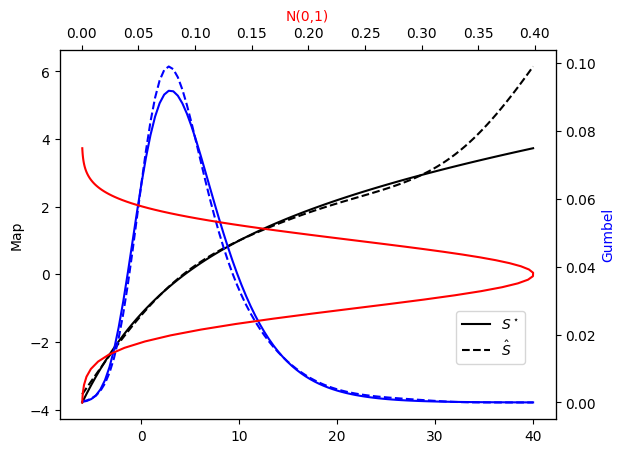
We can now check the accuracy of \(L^\sharp \hat{S}^\sharp \rho \approx \pi\) …

SL = MAPS.CompositeTransportMap(S,L)
pull_SL_rho = DIST.PullBackTransportMapDistribution(SL, rho)
plot_mapping(pi, Sstar, pull_SL_rho, SL)